Using multiRF for Multi-Omics Integration

Overview

multiRF integrates matched multi-omics data with directed multivariate random forests. The current workflow has four main stages:

fit one forest for each requested response–predictor block direction;
construct and fuse sample-level forest weight matrices;
separate shared from block-specific signal and cluster both components;
optionally calculate inverse minimal depth (IMD), select variables, and refit a robust model.

multiRF directly supports multivariate regression, unsupervised residual forests, all-sample and out-of-bag forest weights, ordinary and enhanced proximity, weighted candidate-variable sampling, and depth-based forest IMD. Parts of the implementation, including sampling and random-number-generation routines, are adapted from randomForestSRC under GPL (>= 3). RF-SRC is also available as an optional fallback rather than a requirement for the standard workflow.

This vignette uses a small deterministic subset of the bundled TCGA BRCA data so that every evaluated chunk runs quickly. For an analysis, use all eligible samples, a scientifically justified feature-filtering rule, and more trees (the workflow default is 500).

Input data

The input is a named list of numeric matrices or data frames. Samples are rows and features are columns. Every block must have:

the same number of samples;
identical, unique sample row names in the same order;
unique feature names; and
finite, non-constant numeric features.

Do not pass unordered blocks and rely on their row positions. Align them by sample identifier before fitting. Missing values and categorical predictors should be imputed or encoded explicitly before fitting with multiRF.

full_dimensions <- data.frame(
  block = names(tcga_brca),
  samples = unname(vapply(tcga_brca, nrow, integer(1))),
  features = unname(vapply(tcga_brca, ncol, integer(1)))
)
knitr::kable(full_dimensions)

block	samples	features
gene	674	200
methy	674	200
mirna	674	100


demo_n <- 100L
demo_p <- c(gene = 40L, methy = 40L, mirna = 30L)
demo_ids <- rownames(tcga_brca[[1L]])[seq_len(demo_n)]

brca_demo <- lapply(names(tcga_brca), function(block) {
  x <- tcga_brca[[block]]
  x[demo_ids, seq_len(min(demo_p[[block]], ncol(x))), drop = FALSE]
})
names(brca_demo) <- names(tcga_brca)

stopifnot(all(vapply(
  brca_demo,
  function(x) identical(rownames(x), demo_ids),
  logical(1)
)))

knitr::kable(data.frame(
  block = names(brca_demo),
  samples = unname(vapply(brca_demo, nrow, integer(1))),
  features = unname(vapply(brca_demo, ncol, integer(1)))
))

block	samples	features
gene	100	40
methy	100	40
mirna	100	30

filter_mode = "auto" is the default and performs an omics-aware dispersion prefilter before any forest is fitted. Here the bundled matrices are already curated and then deliberately subset, so the example uses filter_mode = "none". This input prefilter is distinct from IMD-based variable selection later in the workflow.

A complete, fast example

mrf3() is the compact user-facing entry point. In this example it fits all directed forests, constructs the shared and specific components, calculates raw IMD, and applies the mixture selector without a second forest fit.

fit <- mrf3(
  dat.list = brca_demo,
  k = NULL,
  ntree = 40,
  filter_mode = "none",
  main_clustering = "similarity",
  run_imd = TRUE,
  run_variable_selection = TRUE,
  variable_selection_args = list(
    method = "mixture",
    signal = "shared",
    level = 0.05,
    re_fit = FALSE
  ),
  return_data = TRUE,
  nthread = 1,
  filter_verbose = FALSE,
  verbose = FALSE,
  seed = 529
)

With k = NULL, cluster number is selected from the learned representation without using the clinical annotations introduced later. The mixture rule keeps this vignette fast. The adaptive OOB filtering rule is described in Variable selection.

summary(fit)
#> mrf3_fit Summary
#> ---------------- 
#>   Blocks      : 3
#>   Block names : gene, methy, mirna
#>   Samples     : 100
#>   Models      : 6
#>   Connections : 6
#> 
#>   Top-v: model=28, fused=37
#> 
#> Branches
#>   - shared: ran (computed shared weights and shared clustering)
#>   - specific: ran (specific=Spectral)
#>   - imd: ran (net=0)
#>   - cluster_imd: skipped (skipped)
#>   - variable_selection: ran (method=mixture, p_selected=6/15/7)
#>   - robust_clustering: skipped (skipped)
#> 
#> Shared Fraction (top blocks)
#>   data shared_frac specific_ratio           method
#>  methy       0.311          0.689 signal_frobenius
#>   gene       0.296          0.704 signal_frobenius
#>  mirna       0.278          0.722 signal_frobenius

fit_overview <- data.frame(
  quantity = c(
    "directed forests", "model top-v", "fused top-v",
    "shared clusters", "selected variables"
  ),
  value = c(
    length(get_models(fit)),
    fit$model_top_v,
    if (is.null(fit$fused_top_v)) "none" else fit$fused_top_v,
    length(unique(get_clusters(fit))),
    sum(vapply(get_selected_vars(fit), length, integer(1)))
  )
)
knitr::kable(fit_overview)

quantity	value
directed forests	6
model top-v	28
fused top-v	37
shared clusters	3
selected variables	28

The most useful accessors avoid depending on the internal list layout:

head(get_clusters(fit))
#> [1] 1 2 2 2 2 2
table(shared_cluster = get_clusters(fit))
#> shared_cluster
#>  1  2  3 
#> 17 50 33

specific_cluster_counts <- vapply(
  names(brca_demo),
  function(block) length(unique(get_clusters(fit, block = block))),
  integer(1)
)
specific_cluster_counts
#>  gene methy mirna 
#>     3     2     2

get_top_vars(fit, n = 5)
#> $gene
#>   variable    weight
#> 1     TFF1 0.2368899
#> 2     EDN3 0.2335565
#> 3    VGLL1 0.2190179
#> 4    FABP7 0.1910020
#> 5  C1orf64 0.1853795
#> 
#> $methy
#>     variable    weight
#> 1 cg20415486 0.1838194
#> 2 cg13879483 0.1725670
#> 3 cg20693607 0.1719866
#> 4 cg21941030 0.1695833
#> 5 cg27260772 0.1672297
#> 
#> $mirna
#>       variable    weight
#> 1 MIMAT0000267 0.2674107
#> 2 MIMAT0004603 0.2493576
#> 3 MIMAT0000073 0.2059003
#> 4 MIMAT0000226 0.2052778
#> 5 MIMAT0004509 0.1708929
get_vs_summary(fit)
#>   block p_total p_selected selected_ratio
#> 1  gene      40          6      0.1500000
#> 2 methy      40         15      0.3750000
#> 3 mirna      30          7      0.2333333

Other commonly used accessors are get_models(), get_connection(), get_weights(), get_selected_vars(), and get_data(). Use get_clusters(fit, block = "gene") for a block-specific partition and get_clusters(fit, which = "robust") after running the robust branch.

Directed forests and connections

A connection is stored as c(response, predictor): the second block supplies the split variables and the first supplies the multivariate responses. With three blocks, the default retains all six directed pairwise forests.

connections <- get_connection(fit)
connection_table <- do.call(rbind, lapply(connections, function(x) {
  data.frame(response = x[[1L]], predictor = x[[2L]])
}))
rownames(connection_table) <- NULL
knitr::kable(connection_table)

response	predictor
gene	methy
gene	mirna
methy	gene
methy	mirna
mirna	gene
mirna	methy

Set select_connection = TRUE only when direction screening is intentionally part of the analysis. Otherwise all directed models are retained and their connection scores enter the fusion weights.

For the multiRF multivariate-regression forests, important workflow defaults are:

Setting	Default	Meaning
`ntree`	500 in `mrf3()`	Trees per directed forest
`samptype`	`"swor"`	Approximately 63.2% of samples without replacement
`mtry`	`ceiling(p / 3)`	Candidate predictor variables per split
`ytry`	`ceiling(q / 3)`	Candidate response variables per split
`nsplit`	10	Random populated cut points per candidate variable; use 0 to scan all
`nodesize`	5	Regression terminal-node size setting
`forest.wt`	`"all"`	All-sample weights for reconstruction
`seed`	529	Positive, reproducible seed

At each node, candidate responses are standardized within that node before their component split statistics are combined. The response with the largest component statistic is stored as the multivariate splitting response variable (MSRV). IMD, however, is a forest-level depth measure: for each tree it uses 1 / (minimum split depth + 1) and then averages across trees.

Forest-weight fusion and shared/specific signal

For each directed model, the workflow starts from its sample-by-sample forest weight matrix. The default similarity path then:

removes self weights;
applies model-level top-v truncation and row normalization;
normalizes connection scores within each response block;
averages the response-level matrices uniformly; and
optionally applies fused top-v truncation and row normalization.

The corresponding operations are written explicitly below. Let $F_m$ be the raw forest-weight matrix for directed model $m$ , let $\mathcal{T}_v$ retain the top- $v$ entries in each row (including ties at the cutoff), and let $\mathcal{R}$ denote row normalization. Model-level preprocessing is

$A_{m,ij} = \begin{cases} F_{m,ij}/\max\{1-F_{m,ii},\varepsilon\}, & i \ne j,\\ 0, & i=j, \end{cases} \qquad W_m = \mathcal{R}\!\left\{\mathcal{T}_{v_m}(A_m)\right\}.$

For response block $k$ , define $\mathcal{M}^{(k)}=\{m:\operatorname{response}(m)=k\}$ . If $q_m$ is the connection score, the within-response weights and fused matrix are

$\begin{aligned} s_m &= \begin{cases} [\max\{q_m,c\}]^\gamma, & \text{weighted fusion},\\ 1, & \text{uniform fusion}, \end{cases}\\ \alpha_{km} &= \frac{s_m}{\sum_{r\in\mathcal{M}^{(k)}}s_r}, \qquad W^{(k)} = \mathcal{R}\!\left( \sum_{m\in\mathcal{M}^{(k)}}\alpha_{km}W_m \right). \end{aligned}$

The default global fusion then averages the $K$ response-level matrices before the optional fused top- $v$ step:

$\overline{W}=\frac{1}{K}\sum_{k=1}^{K}W^{(k)}, \qquad W_{\mathcal{M}^*} =\mathcal{R}\!\left\{\mathcal{T}_{v_f}(\overline{W})\right\}.$

Thus, model-level preprocessing feeds within-response fusion, followed by across-response fusion. Weighted fusion uses the connection modularity by default, with $c=0$ and $\gamma=1$ ; if all scores in a response block are invalid or non-positive, the default fallback is uniform weighting. A tuned or fixed top-v at least 80% of the sample size is interpreted as no truncation. model_top_v = Inf and fused_top_v = Inf also request no truncation explicitly; without fused truncation, $\mathcal{T}_{v_f}$ in the across-response formula is the identity.

When model_top_v or fused_top_v is left NULL, the workflow selects it from the mean normalized row entropy of the fused weight matrix, which rises monotonically with $v$ and saturates at the no-truncation value. The default top_v_method = "saturation" keeps the smallest $v$ whose entropy reaches top_v_tau (default 0.9) of that limit, interpolating linearly between candidates so the choice does not depend on the grid resolution; model_top_v is selected first and fused_top_v conditional on it, with the fused curve obtained in closed form for every integer $v$ . The full entropy-versus- $v$ tables are stored in fit$tuning_detail for reporting. top_v_method = "entropy_elbow" (the earlier small-gain elbow heuristic) and "neff" (effective neighbourhood size, no grid) remain available.

The shared and residual-specific affinities are constructed as S = W %*% t(W), with the diagonal set to zero. Spectral clustering is the default similarity backend.

W <- fit$reconstruction$W$W_all
S_shared <- fit$shared$clustering$similarity

c(
  minimum_weight_row_sum = min(rowSums(W)),
  maximum_weight_row_sum = max(rowSums(W)),
  maximum_similarity_diagonal = max(abs(diag(S_shared)))
)
#>      minimum_weight_row_sum      maximum_weight_row_sum maximum_similarity_diagonal 
#>                           1                           1                           0

fit$shared$frac[, c("data", "shared_frac", "specific_ratio")]
#>    data shared_frac specific_ratio
#> 1  gene   0.2963977      0.7036023
#> 2 methy   0.3110102      0.6889898
#> 3 mirna   0.2784850      0.7215150

For block k, the response-specific forest weight matrix gives the shared reconstruction Xhat^(k) = W^(k) X^(k) and the residual R^(k) = X^(k) - Xhat^(k). An unsupervised forest is then fitted to each residual matrix to obtain its block-specific weight matrix and similarity. The reported shared_frac is 1 - ||R^(k)||_F^2 / ||X^(k)||_F^2. It is a descriptive signal fraction, not a hypothesis-test p-value.

Variable selection

Set run_imd = TRUE when global raw IMD should be retained without running a selection branch. run_variable_selection = TRUE and run_robust_clustering = TRUE compute the required IMD automatically. The three IMD selection methods all operate on the unnormalized [0, 1] scale:

Method	Selection rule	When to use it
`"filter"`	For shared IMD, tune `tau * sd(IMD)` with true OOB normalized MSE; for residual-specific IMD, select above a permutation-null quantile	Adaptive forest-based screening; most computationally intensive
`"transformation"` (`"test"`)	Standardize each feature’s forest IMD relative to the block-wide IMD distribution; retain upper-tail features at the chosen `level`, combined by majority vote across connected forests	Distribution-normalized screening
`"mixture"`	Explicit point mass at zero plus two components on positive IMD	Posterior noise-probability selection

method = "thres" is also available when a fixed se * sd(IMD) cutoff is needed. normalized = FALSE is the default because selection is performed on raw IMD. If re_weights = TRUE, the retained raw IMD values are used as multiRF candidate-variable sampling weights during refitting.

The evaluated example used the mixture rule:

get_vs_summary(fit)
#>   block p_total p_selected selected_ratio
#> 1  gene      40          6      0.1500000
#> 2 methy      40         15      0.3750000
#> 3 mirna      30          7      0.2333333
lapply(get_selected_vars(fit), utils::head)
#> $gene
#> [1] "FABP7"   "KLK11"   "EDN3"    "TFF1"    "VGLL1"   "C1orf64"
#> 
#> $methy
#> [1] "cg27260772" "cg01893212" "cg13251533" "cg20399616" "cg08435683" "cg23179456"
#> 
#> $mirna
#> [1] "MIMAT0000226" "MIMAT0001635" "MIMAT0000267" "MIMAT0004603" "MIMAT0000073"
#> [6] "MIMAT0000754"

Plots from an mrf3_fit object use the unified plot(fit, type = ...) interface. Recommended types are "tsne", "umap", "network", "circos", "composition", "km", and "weights"; additional arguments are forwarded to the corresponding plot implementation.

IMD values can be inspected independently of the selected set:

plot(fit, type = "weights", weight_source = "imd", top = 8)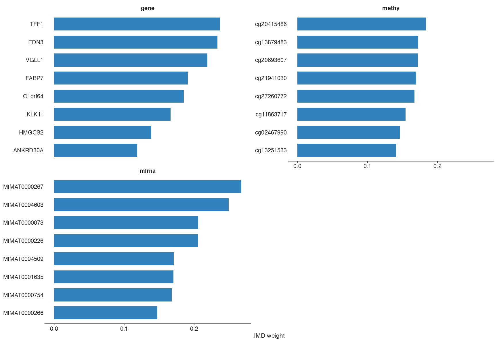

For the shared-signal adaptive OOB filter, use:

vs_filter <- mrf3_vs(
  mod = fit,
  method = "filter",
  signal = "shared",
  k = 3,
  tol = 0.01,
  re_fit = FALSE
)
get_selected_vars(vs_filter)

The filter is signal-specific: shared IMD uses the OOB search, while residual-specific IMD uses the perm_quantile of pooled IMD values from perm_B column-wise permutation refits. With signal = "all", the workflow returns the union of these selections. The specific filter requires the residual matrices retained by mrf3_fit(); if they are unavailable, it warns and uses the fixed cutoff. The transformation and mixture methods can be applied directly to signal = "shared", "specific", or "all".

vs_transformation <- mrf3_vs(
  fit, method = "transformation", signal = "shared",
  level = 0.05, re_fit = FALSE
)

vs_union <- mrf3_vs(
  fit, method = "mixture", signal = "all",
  level = 0.05, re_fit = FALSE
)

Standalone mrf3_vs() defaults to re_fit = TRUE. The staged workflow does not refit unless requested, except that run_robust_clustering = TRUE must and therefore does force a final refit.

Clustering modes and PAM50 annotation

The main_clustering argument applies the same representation choice to the shared and specific branches:

Mode	Representation	Default clustering backend
`"similarity"`	`W W^T` from fused or residual weights	Spectral
`"proximity"`	Same-terminal-node frequency	PAM
`"enhanced_proximity"`	Proximity plus sibling-leaf correction	PAM

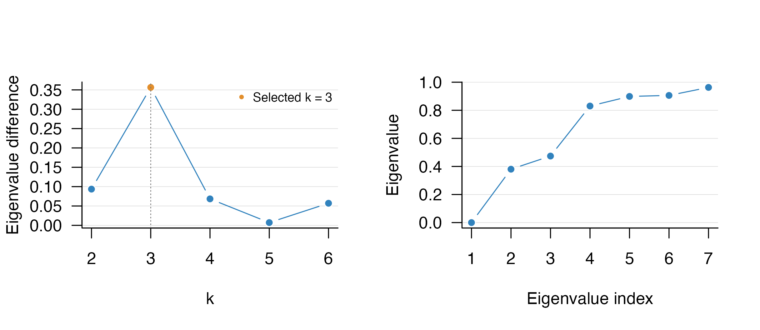
The evaluated fit selected three shared clusters by the eigengap of its learned similarity. The diagnostic below repeats that calculation over k = 2, ..., 6. It is retrospective to the fit and does not use PAM50 or any other clinical annotation.

k_diagnostic <- tune_k_clusters(
  S_shared,
  method = "Spectral",
  k_tune = 2:6,
  return_cluster = TRUE,
  plot_k = TRUE
)

stopifnot(k_diagnostic$best_k == length(unique(get_clusters(fit))))

Post hoc comparison with PAM50

PAM50 is used here only after fitting to annotate the unsupervised shared partition. It was not supplied to feature selection, forest construction, weight fusion, cluster-number tuning, or clustering. Because PAM50 itself is derived from gene expression and gene expression is one of the multiRF input blocks, this is a biological concordance check rather than an independent ground truth.

All 94 primary tumors in the demonstration subset had a PAM50 call. The remaining 6 adjacent-normal samples had no tumor-subtype label and are excluded from this comparison. The same t-SNE coordinates are used in panels a and b; only the coloring changes. Panels a and b use plot(..., type = "tsne"), and panel c uses plot(..., type = "composition") to show the exact within-cluster composition. All three panels use the unified plotting interface; the assembly code is hidden here to keep the vignette concise.

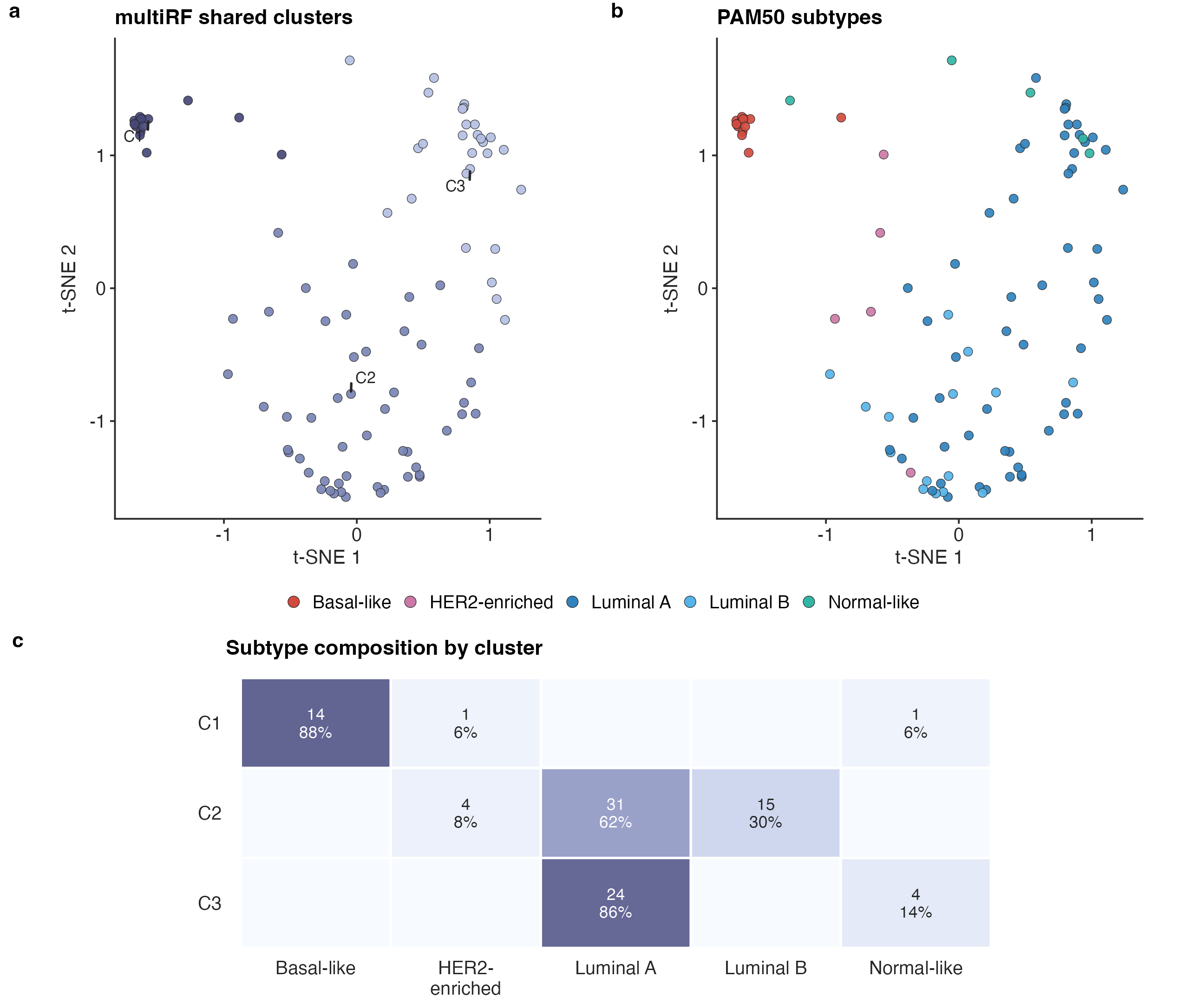
Relationship between the multiRF shared partition and PAM50 annotations in the demonstration subset. (a, b) The same t-SNE embedding of the learned shared similarity for 94 primary tumors, colored by multiRF cluster (a) or PAM50 annotation (b). t-SNE is used only for visualization. (c) Within-cluster PAM50 composition; labels show sample count and row percentage.

The three-cluster partition captures a coarse organization of PAM50-related biology rather than a one-to-one recovery of five subtypes: C1 is almost entirely Basal-like, whereas C2 and C3 divide the luminal-rich samples. The agreement metrics are reported below. Fixing five clusters on the same learned similarity is included only as a sensitivity analysis and does not improve agreement.

knitr::kable(pam50_metrics, digits = 3)

resolution	n	ari	jaccard	nmi	purity
Unsupervised k = 3	94	0.267	0.383	0.497	0.734
Fixed k = 5 sensitivity	94	0.213	0.282	0.443	0.734

The similarity workflow is the default. To compare representations on a full analysis, keep the data, tree settings, and positive seed fixed:

fit_similarity <- mrf3(
  dat.list, k = 4, ntree = 500,
  main_clustering = "similarity", seed = 529
)

fit_proximity <- mrf3(
  dat.list, k = 4, ntree = 500,
  main_clustering = "proximity", seed = 529
)

fit_enhanced <- mrf3(
  dat.list, k = 4, ntree = 500,
  main_clustering = "enhanced_proximity", seed = 529
)

If k = NULL, cluster number is tuned in the downstream clustering stage, as in the evaluated fit. For a fixed biological hypothesis, supply k explicitly. tune_k_clusters() draws its diagnostic on the active graphics device and restores the prior base-graphics settings afterward.

The ggplot objects returned by the unified interface can be composed or exported at final figure size. For example, ggplot2::ggsave("shared-tsne.pdf", width = 85, height = 75, units = "mm") writes a vector figure; use TIFF or PNG at 600 dpi when a raster file is required. The default sans family is portable across R devices.

Robust and cluster-specific analyses

Robust clustering repeats reconstruction after feature selection. It is an optional, more expensive branch:

fit_robust <- mrf3(
  dat.list,
  k = 4,
  ntree = 500,
  run_imd = TRUE,
  run_variable_selection = TRUE,
  run_robust_clustering = TRUE,
  variable_selection_args = list(
    method = "filter",
    re_weights = TRUE
  ),
  seed = 529
)

table(get_clusters(fit_robust, which = "robust")$shared)

Cluster-specific IMD is separate from global IMD and must be requested explicitly:

fit_cluster_imd <- mrf3(
  dat.list,
  k = 4,
  ntree = 500,
  run_imd = TRUE,
  run_cluster_imd = TRUE,
  cluster_imd_args = list(min_cluster_size = 15),
  seed = 529
)

get_weights(fit_cluster_imd$cluster_imd, cluster = 1)

Reproducibility and resource use

Use a non-negative integer seed for a reproducible multiRF fit; 529 is the package default. A negative seed deliberately requests system entropy. Reproducible seeds give the same result across thread counts.
Set options(multiRF.nthread = n) or pass nthread = n to control parallel tree construction.
Keep samptype = "swor" for the default workflow. Sampling with replacement is supported when it is scientifically intended.
Forest weights and proximity matrices are n by n. For large cohorts, account for these matrices when choosing worker counts.
compact_output = TRUE reduces retained duplicate objects, but do not use it when models will be needed for later custom reconstruction or reclustering.
Record packageVersion("multiRF"), the random seed, connections, tree settings, selected top-v values, and clustering arguments with every result.

For a production fit without automatic input prefiltering:

options(multiRF.engine = "native", multiRF.nthread = 4L)

fit_final <- mrf3_fit(
  dat.list = dat.list,
  ntree = 500,
  samptype = "swor",
  filter_mode = "none",
  main_clustering = "similarity",
  clustering_args = list(shared_k = 4, specific_k = 2),
  top_v_method = "saturation",
  select_connection = FALSE,
  run_imd = TRUE,
  run_variable_selection = TRUE,
  variable_selection_args = list(
    method = "filter",
    signal = "shared",
    k = 3,
    re_fit = FALSE
  ),
  return_data = TRUE,
  seed = 529
)

Common problems

Rows are silently mismatched. They should not be: current validation stops on unequal or reordered sample identifiers. Align every block explicitly.

A constant feature becomes non-finite after scaling. Remove constant and non-finite columns before fitting, or use an appropriate filtering mode.

mrf3_vs() cannot find data. Supply dat.list directly or fit with return_data = TRUE.

A response block is absent from reconstruction. Per-response fusion requires at least one fitted response-side connection for every input block; the workflow now stops rather than substituting a global matrix.

Block names contain underscores. Current fits retain explicit response and predictor metadata, so underscores are supported. Avoid parsing model display names in downstream code; use get_connection().

Citation

If you use multiRF, please cite the method relevant to your analysis:

Zhang, W., Wang, L., Franzmann, E. J., and Chen, X. S. (2026). Multivariate Random Forests for Cross-Modal Multi-Omics Integration. bioRxiv. doi:10.64898/2026.06.17.732933

Zhang, W. et al. (2025). An integrative multi-omics random forest framework for robust biomarker discovery. GigaScience, 14, giaf148. doi:10.1093/gigascience/giaf148

multiRF adapts parts of randomForestSRC and also supports it as an optional fallback; please also cite:

Ishwaran, H., and Kogalur, U. B. (2026). randomForestSRC: Fast Unified Random Forests for Survival, Regression, and Classification (RF-SRC). R package version 3.6.2. doi:10.32614/CRAN.package.randomForestSRC

Ishwaran, H., and Kogalur, U. B. (2007). Random survival forests for R. R News, 7(2), 25–31. Article

Session information

packageVersion("multiRF")
#> [1] '0.3.0'
sessionInfo()
#> R version 4.6.0 (2026-04-24)
#> Platform: aarch64-apple-darwin23
#> Running under: macOS Tahoe 26.6.2
#> 
#> Matrix products: default
#> BLAS:   /Library/Frameworks/R.framework/Versions/4.6/Resources/lib/libRblas.0.dylib 
#> LAPACK: /Library/Frameworks/R.framework/Versions/4.6/Resources/lib/libRlapack.dylib;  LAPACK version 3.12.1
#> 
#> locale:
#> [1] C.UTF-8/C.UTF-8/C.UTF-8/C/C.UTF-8/C.UTF-8
#> 
#> time zone: America/New_York
#> tzcode source: internal
#> 
#> attached base packages:
#> [1] stats     graphics  grDevices utils     datasets  methods   base     
#> 
#> other attached packages:
#> [1] multiRF_0.3.0
#> 
#> loaded via a namespace (and not attached):
#>  [1] sass_0.4.10        generics_0.1.4     tidyr_1.3.2        rstatix_1.1.0     
#>  [5] digest_0.6.39      magrittr_2.0.5     evaluate_1.0.5     grid_4.6.0        
#>  [9] RColorBrewer_1.1-3 fastmap_1.2.0      jsonlite_2.0.0     ggrepel_0.9.8     
#> [13] backports_1.5.1    Formula_1.2-6      purrr_1.2.2        scales_1.4.0      
#> [17] textshaping_1.0.5  jquerylib_0.1.4    abind_1.4-8        cli_3.6.6         
#> [21] rlang_1.3.0        cowplot_1.2.0      withr_3.0.2        cachem_1.1.0      
#> [25] yaml_2.3.12        otel_0.2.0         tools_4.6.0        ggsignif_0.6.4    
#> [29] dplyr_1.2.1        ggplot2_4.0.3      ggpubr_1.0.0       broom_1.0.13      
#> [33] vctrs_0.7.3        R6_2.6.1           lifecycle_1.0.5    fs_2.1.0          
#> [37] car_3.1-5          htmlwidgets_1.6.4  ragg_1.5.2         cluster_2.1.8.2   
#> [41] pkgconfig_2.0.3    desc_1.4.3         pkgdown_2.2.1      pillar_1.11.1     
#> [45] bslib_0.11.0       gtable_0.3.6       glue_1.8.1         Rcpp_1.1.1-1.1    
#> [49] systemfonts_1.3.2  xfun_0.58          tibble_3.3.1       tidyselect_1.2.1  
#> [53] knitr_1.51         farver_2.1.2       htmltools_0.5.9    igraph_2.3.3      
#> [57] carData_3.0-6      rmarkdown_2.31     labeling_0.4.3     compiler_4.6.0    
#> [61] S7_0.2.2

Wei Zhang